Mitochondria Skeleton Length Calculator (Matlab)

You can download the .m file here and install it as an app to access the function.

The Terms

Bounding Box

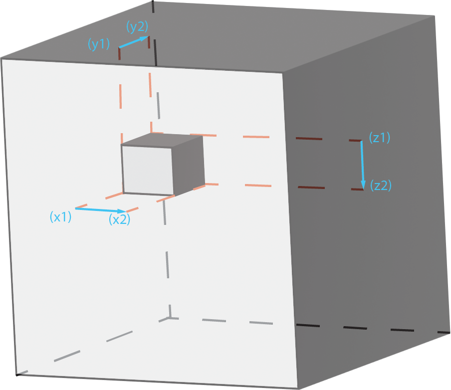
A bounding box of a section is decided by its largest and smallest values in x, y, and z direction. The length, width, and height of a bounding box can be obtained by doing subtractions bewteen each pair of x, y, and z values.

Here is an example of a bounding box in the total volume:

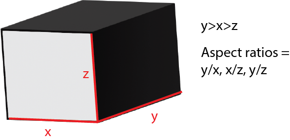
Aspect Ratio

The aspect ratio the ratio between the length and width of a shape. Since the bounding box of a section is a rectangular prism, this project takes 3 aspect ratio of each section: xy, xz, yz.

Skeleton

The skeleton of sections is obtained using the skeleton3d function. The process of “skeletonization” is also known as the Medial Axis Transform. Detailed examples of 3d skeletonization can be found here, an alternative to skeleton3d. However, neither of these two functions calculates the length of the generated skeletons. Therefore, calculating the length of skeletons became the goal for this program.

Connectivity

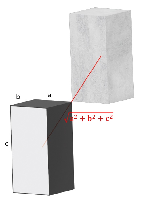
In order to calculate the length of the generated skeleton, this program calculate the distance between each adjacent voxel and add them up. In a 3d space, one voxel can have 26 distinct adjacent voxels surrounding it. These 26 can be classified to 3 categories: connected via surface, via edge, and via point. The 3 categories each have different method to obtain the distance between the two voxels.

Connected surface (6 total, devided to 3 kinds):

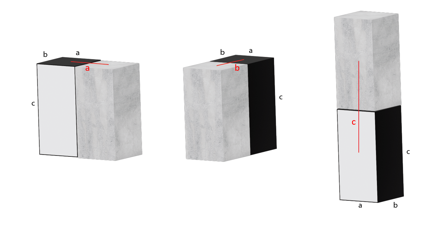
Connected edge (12 total, devided to 3 kinds):

Connected point (8 total):

The Codes

How to use

The function takes 7 inputs: mito_meta_file_name, pixel_length, pixel_width, page_thickness, shrinked_ratio, sample_name, and full__h5_directory. Since the h5 file is exported as 2048/2048pixels resolution, the resolution can be different from the original image volume. The “shrinked_ratio” is simply origianl image volume length/2048. The rest of the inputs are pretty self explanitory. An example would be:

mito_skel_length_aspect_ratio_calculator('mouse_mito_meta',16,16,40,2,'mouse','C:\mito_project\mouse_h5_folder\mouse_mito_16nm.h5')

Getting Started

First, access the cvs file and extract index and bounding box coordinates, and convert them to 2 arrays.

mito_meta = readtable(mito_meta_file_name);
mito_index = table2array(mito_meta(:,1));
bbox_array = table2array(mito_meta(:,19:24));

Next, remove the categorical parent sections, which only serve as folders for other sections and are not actually drawn. The bounding box values for these sections are all -1.

probelm = [-1 -1 -1 -1 -1 -1];
while ismember(probelm,bbox_array,'rows') == 1
    rowindex = find(ismember(bbox_array,probelm,'rows')>0);
    bbox_array(rowindex(1),:)=[];
    mito_index(rowindex(1),:)=[];
end

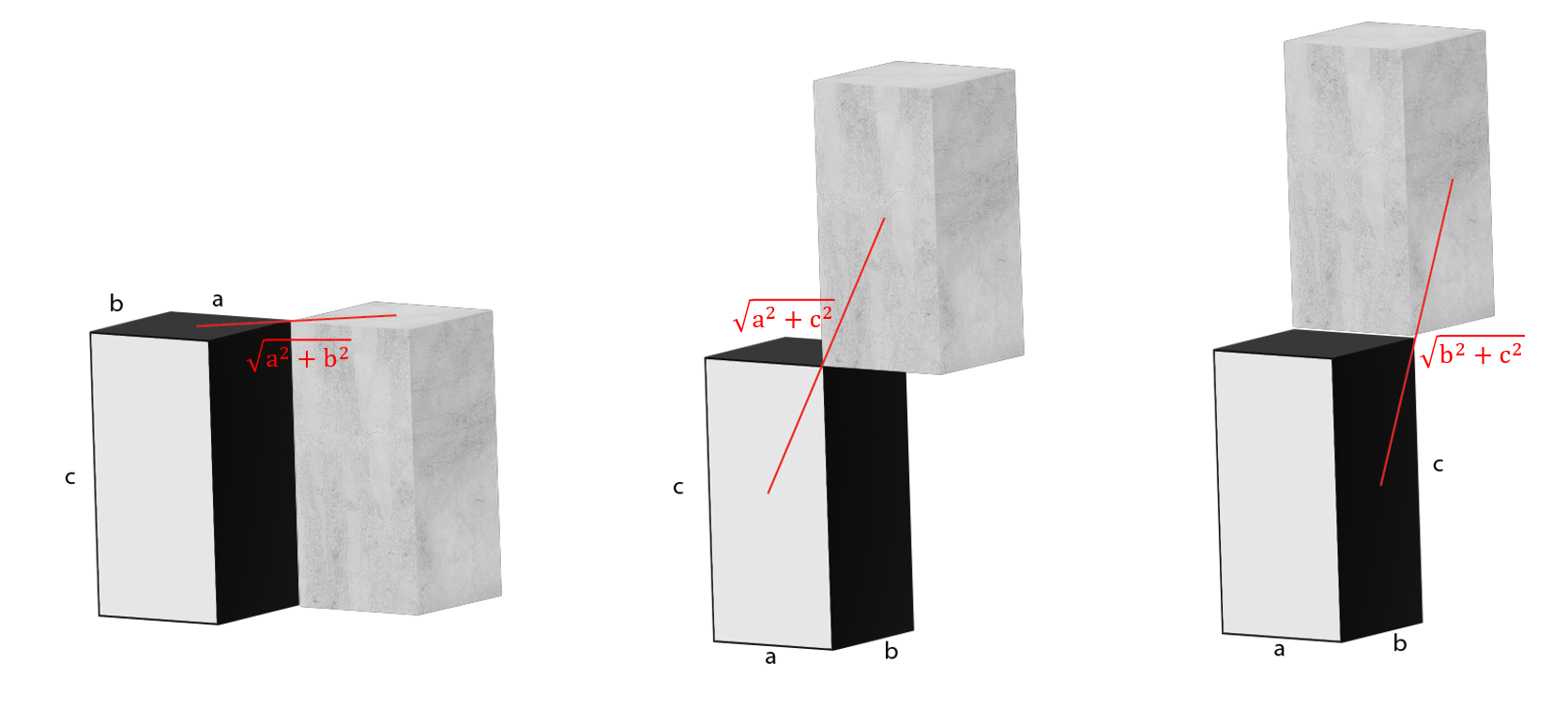
Also calculate the potential distancse in nanometers between two adjacent voxels, based on pixel length, pixel width, page thickness, and connectivity.

voxel_length = pixel_length*shrinked_ratio; 
voxel_width = pixel_width*shrinked_ratio; 
voxel_height = page_thickness; 
edge_dist_a = sqrt(voxel_length^2+voxel_width^2);
edge_dist_b = sqrt(voxel_length^2+voxel_height^2);
edge_dist_c = sqrt(voxel_width^2+voxel_height^2);
point_dist = sqrt(voxel_length^2+voxel_width^2+voxel_height^2);

Aspect Ratio

Calculation Function:

Each ratio is calculated with the larger value devided by the smaller value.

  function d = get_ratio(a,b)
        if a>b
            d = a/b;
        else
            d = b/a;
        end
    end

Getting Aspect Ratios

This program calculates the aspect ratios of the bounding boxes and not the mitochondria themselves. And the lengths, widths, and heights of the bounding boxes can be mathmetically calculated with the data provided by mito_meta.

Since the bounding box’s side lengths are number of pixels, to calculate the true ratio of each mitochondria, the x length needed to be multiplied with pixel_length, as the y length with pixel_width and z length with page_thickness. After the calculation of each bounding box, the 3 aspect ratios are appended to an array as a vector.

x_true_dist = (bbox_array(index,4)-bbox_array(index,1))*pixel_length;
y_true_dist = (bbox_array(index,5)-bbox_array(index,2))*pixel_width;
z_true_dist = (bbox_array(index,6)-bbox_array(index,3))*page_thickness;
xy_ar = get_ratio(x_true_dist,y_true_dist);
xz_ar = get_ratio(x_true_dist,z_true_dist);
yz_ar = get_ratio(y_true_dist,z_true_dist);
aspect_ratios = [aspect_ratios;
                  [mito_index(index) xy_ar xz_ar yz_ar]];

Skeleton Length

Extracting the Boundary Box and Generating the Skeleton

Reading the full h5 file is way too much work. Therefore, for each mitochondrion, this program only read the part of the h5 defined by the mitochondrion’s bounding box. Also due to the sheer sizes of h5 files, the image stacks are shrinked from their origin dimentions to (2048 pixel x 2048 pixel x original page number). Therefore, to find the start and distance in the h5 files, this program needs to devide the data from mito_meta with the shrinked ratio, or else the h5read() would have exceed limit errors. Since the h5 files are generated with a python program, whose index starts with 0, this program, a matlab program, whose index starts with 1, need to +1 to the values to eliminate 0 values.

The approximate bounding box, which is a 3d array, needs to be binarized according to the greyscale index of the mitochondrion in each loop, since skeletonization can only be used in binarized arrays/images. Afterwards, the skeleton of the mitochondrion can be generated with just a single line of code.

x_start = floor(bbox_array(index,1)/shrinked_ratio)+1;
y_start = floor(bbox_array(index,2)/shrinked_ratio)+1;
z_start = bbox_array(index,3)+1;
x_distance = floor((bbox_array(index,4)-bbox_array(index,1))/shrinked_ratio)+1;
y_distance = floor((bbox_array(index,5)-bbox_array(index,2))/shrinked_ratio)+1;
z_distance = bbox_array(index,6)-bbox_array(index,3)+1;
start = [x_start y_start z_start];
count =[x_distance y_distance z_distance];
bbox = h5read(full__h5_directory,'/images',start,count);
%binarize the content within boundary box, removing all content other than the selected mito, according to grey value
bi_bbox = bbox == mito_index(index);
%make the skeleton of the mito
skel = Skeleton3D(bi_bbox);

Slicing Branches

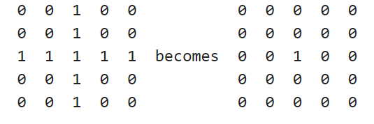
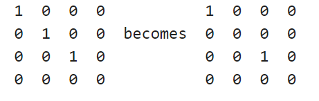
As mentioned before, the length of a skeleton is calculated by adding the distances between each adjacent voxels. However, how does the program determine where to start, and when to stop? Fortunately, in the bwmorph3 function, there are 2 concepts that are very helpful: branch points, and end points. Essencially, branch poitns are voxels that have 3 or more adjacent voxels who are also in the skeleton, and end points are voxels that only have 1 adjacent voxel that is in the skeleton. Here are examples of branch points and end points in 2d from bwmorph:

Branch Point:

End Point:

First, the program finds the coordinates of all the branch points, and change the 1s in those coordinates into 0s. This removes the points from the skeleton, which is now sliced into branches.

%find branch points and their coordinates
Bpoints = bwmorph3(skel,'branchpoints');
Bpoints_c = [];
[row, col, page] = findND(Bpoints == 1);
for i = length(row)
    Bpoints_c = [Bpoints_c; [row, col, page]];
end
%slicing branches
branches = skel - Bpoints;

Then, find the coordinates of endpoints of every branch and append them in an array as vectors.

Epoints = bwmorph3(branches,'endpoints');
Epoints_c = [];
[row, col, page] = findND(Epoints == 1);
for i = length(row)
    Epoints_c = [Epoints_c; [row, col, page]];
end

Since each branch has 2 end points, the length of Epoints_c is always even, and the coordinates in it can always be paired up.

Last but not least, find the coordinates of all points in all branches

skel_c = [];
[row, col, page] = findND(branches == 1);
for i = length(row)
    skel_c = [skel_c; [row, col, page]];
end

Now that the program have all the necessary component, it can start the calculation of the length of the skeleton!

Skeleton Length Calculation

The program starts the calculation at the first end point in endpoint_c, registering the point as start_point and removing its coordinate from both arrays of coordinates: skel_c and Epoint_c, to avoid repetition .

start_point = Epoints_c(1,:);
skel_c(find(ismember(skel_c, start_point,'rows')),:) = [];
Epoints_c(find(ismember(Epoints_c, start_point,'rows')),:) = [];

Then, the program finds the coordinate of every voxel surrounding start_point. When I wrote the code, I separted p1~p26 by layers.

p1 = [start_point(1)-1, start_point(2)-1, start_point(3)-1];
p2 = [start_point(1), start_point(2)-1, start_point(3)-1];
p3 = [start_point(1)+1, start_point(2)-1, start_point(3)-1];
p4 = [start_point(1)-1, start_point(2), start_point(3)-1];
p5 = [start_point(1), start_point(2), start_point(3)-1];
p6 = [start_point(1)+1, start_point(2), start_point(3)-1];
p7 = [start_point(1)-1, start_point(2)+1, start_point(3)-1];
p8 = [start_point(1), start_point(2)+1, start_point(3)-1];
p9 = [start_point(1)+1, start_point(2)+1, start_point(3)-1];

p10 = [start_point(1)-1, start_point(2)-1, start_point(3)];
p11 = [start_point(1), start_point(2)-1, start_point(3)];
p12 = [start_point(1)+1, start_point(2)-1, start_point(3)];
p13 = [start_point(1)-1, start_point(2), start_point(3)];
p14 = [start_point(1)+1, start_point(2), start_point(3)];
p15 = [start_point(1)-1, start_point(2)+1, start_point(3)];
p16 = [start_point(1), start_point(2)+1, start_point(3)];
p17 = [start_point(1)+1, start_point(2)+1, start_point(3)];

p18 = [start_point(1)-1, start_point(2)-1, start_point(3)+1];
p19 = [start_point(1), start_point(2)-1, start_point(3)+1];
p20 = [start_point(1)+1, start_point(2)-1, start_point(3)+1];
p21 = [start_point(1)-1, start_point(2), start_point(3)+1];
p22 = [start_point(1), start_point(2), start_point(3)+1];
p23 = [start_point(1)+1, start_point(2), start_point(3)+1];
p24 = [start_point(1)-1, start_point(2)+1, start_point(3)+1];
p25 = [start_point(1), start_point(2)+1, start_point(3)+1];
p26 = [start_point(1)+1, start_point(2)+1, start_point(3)+1];

Then, the program checks whether any of these coordinates are in skel_c, which would imply the voxel being on the skeleton. Since start_point is an end point, there should only be 1 adjacent voxel for start_point. After finding the adjacent voxel, the program adds a certain distance to the float total_distance, based on the connectivity between the adjacent voxel and start_point. Then the coordinate this adjacent voxel is removed from skel_c to avoid repetition. Then start_point is redefined by the coordinates of this adjacent voxel, and start over the loop of calculation.

If the coordinate of this adjacent voxel is in Epoint_c, which would imply the end of a branch, the program would end the current while loop, and continue down the list of Epoint_c, until the array is empty. At which point, all the branches would be calculated, and the total length of the skeleton would be a float total_distance.

The order in which the program checks each of the 26 adjacent voxels is from the closest category of connectivity to the longest category of connectivity: surface, edge, and then point. Since the full code is too long, here is an example code for p5, a voxel connected to start_point through a surface. The rest of the possibilities are written with elseif statements.

if ismember(p5,skel_c,'rows') == 1
    total_length = total_length+voxel_height;
    skel_c(find(ismember(skel_c, p5,'rows')),:) = [];
    if ismember(p5,Epoints_c,'rows') == 1
        Epoints_c(find(ismember(Epoints_c, p5,'rows')),:) = [];
        anymore = 0;
    end
    start_point = p5;

After the distance of every pair of adjacent voxels in every branch is added to total_distance, it is appended to all_skel_lengths, and then reset to 0.

Output

The aspect ratio and skeleton length of every mitochondrion are now in 2 arrays. Not it is time to combine them and output a .csv file, which is the final step of this program.

aspect_ratios(:,5) = all_skel_lengths(:,2);
header = {'index','xy_ratio','xz_ratio','yz_ratio','skel_length'};
output = [header; num2cell(aspect_ratios)];
final_data = cell2table(output(2:end,:),'VariableNames',output(1,:));
file_name = append(sample_name,'_mito_aspect_ratios_skel_length.csv');
writetable(final_data,file_name);